Basic Usage#

Setup#

This tutorial notebook will walk you through the basic usage of the OTTER API. First make sure you followed the installation structions to install otter and the data. First the imports we will need for the notebook

[1]:

import os
import otter

from astropy.coordinates import SkyCoord
from astropy import units as u

import matplotlib.pyplot as plt
import numpy as np

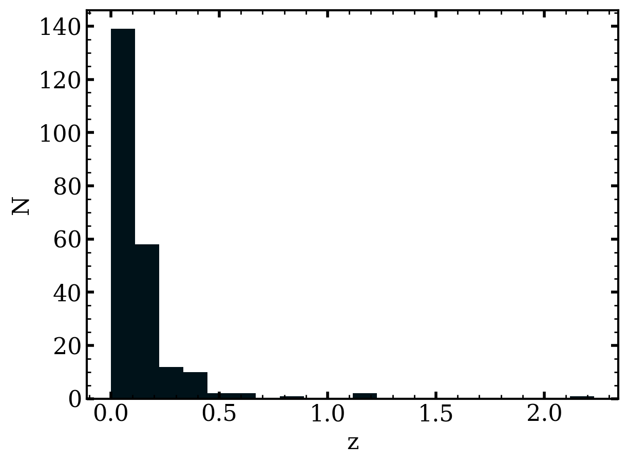
We can initiate the otter database object and then get metadata of all of the data. From there, we can easily get the default redshift for each object and histogram them.

Note: When calling get_meta it does not return the photometry. This is to make metadata queries much quicker. See below for also accessing the photometry along with metadata.

[2]:

db = otter.Otter()
meta = db.get_meta(classification="TDE")
redshifts = np.array([t.get_redshift() for t in meta if "distance" in t and len(t["distance"]) > 0])
fig, ax = plt.subplots()
ax.hist(redshifts.astype(float), bins=20)
ax.set_ylabel("N")
ax.set_xlabel("z")

Attempting to login to https://otter.idies.jhu.edu/api with the following credentials:
username: user-guest
password: test

[2]:

Text(0.5, 0, 'z')

Querying the OTTER Catalog#

Now that we have the catalog read in an initiated, we can query it for the data we want. Say we want to get all of the data associated with the TDE Sw J1644+57, we can use

[3]:

swj1644_list = db.query(names='Sw J1644+57')
swj1644_list

[3]:

[Transient(
        Name: Sw J1644+57,
        Keys: dict_keys(['_key', '_id', '_rev', 'classification', 'name', 'coordinate', 'filter_alias', 'photometry', 'reference_alias', 'distance', 'host', 'date_reference', 'schema_version', '_dec', '_ra'])
 )]

Which you can see is a list of otter Transient objects. You can essentially treat this like a python dictionary with some benefits:

It has additional helpful methods to access and clean the data
You can use the HDF5 slash-syntax. Ex.) swj1644['name/alias'] will give you all of the aliases from the alias subkey in the name key

[4]:

swj1644 = swj1644_list[0] # just to get rid of the list

swj1644['name/alias']

[4]:

[{'value': 'GRB 110328A', 'reference': ['2011Sci...333..203B']},
 {'value': 'Swift J1644+57',
  'reference': ['2017ApJ...838..149A',
   '2011Sci...333..203B',
   '2023PASP..135c4101G']},
 {'value': 'Sw J1644+57', 'reference': ['Swift', '2011Natur.476..425Z']},
 {'value': 'Swift J164449.3+573451', 'reference': ['2011Sci...333..203B']},
 {'value': 'SwJ1644+57',
  'reference': ['2011Natur.476..425Z', '2011Natur.476..425Z']}]

So this TDE has multiple aliases associated with it! Let’s try to query by a different one

[5]:

db.query(names='GRB 110328A')[0]

[5]:

Transient(
        Name: Sw J1644+57,
        Keys: dict_keys(['_key', '_id', '_rev', 'classification', 'name', 'coordinate', 'filter_alias', 'photometry', 'reference_alias', 'distance', 'host', 'date_reference', 'schema_version', '_dec', '_ra'])
)

And look at that, it gives us the same answer! We can also query by a list of names which will give us a list of transient objects back:

[6]:

db.query(names=['Sw J1644+57', '2018hyz', '2018zr'])

[6]:

[Transient(
        Name: Sw J1644+57,
        Keys: dict_keys(['_key', '_id', '_rev', 'classification', 'name', 'coordinate', 'filter_alias', 'photometry', 'reference_alias', 'distance', 'host', 'date_reference', 'schema_version', '_dec', '_ra'])
 ),
 Transient(
        Name: 2018hyz,
        Keys: dict_keys(['_key', '_id', '_rev', '_dec', '_ra', 'classification', 'coordinate', 'date_reference', 'distance', 'filter_alias', 'name', 'photometry', 'reference_alias', 'schema_version'])
 ),
 Transient(
        Name: 2018zr,
        Keys: dict_keys(['_key', '_id', '_rev', 'reference_alias', 'classification', 'coordinate', 'distance', 'name', 'date_reference', 'host', 'schema_version', 'filter_alias', 'photometry', '_dec', '_ra'])
 )]

We can also search OTTER for anything within a certain redshift range, let’s look for everything between \(0.1 < z <0.2\):

[7]:

len(db.query(minz=0.1, maxz=0.2))

[7]:

WOW! That’s a lot of transients. But that’s expected since many of them are discovered nearby. What if we look for everything with a redshift over 1?

[8]:

len(db.query(minz=1))

[8]:

Ah makes sense, it is just those rarer high redshift events.

Cone Searches#

Moving on from general querys, we can perform cone searches on the catalog using the otter.Otter.cone_search method. Let’s do this for objects within 15 degrees of the ecliptic pole.

[9]:

# first construct a SkyCoord
coord = SkyCoord('18h00m00.0s', '+66d33m38.84s', unit=(u.hourangle, u.deg))
radius = (15*u.deg).to(u.arcsec).value # must just provide it as a float

len(db.cone_search(coord, radius=radius))

[9]:

Sample Selection#

Given that OTTER includes many transients that are only classified based on photometric information, we provide numerous flags for selecting a subsamble of events based on your scientific goals:

spec_classed is True if the event is spectroscopically classified
unambiguous is True if the community unambiguously agrees on this classification
class_confidence_threshold let’s you set a minimum for the “confidence” flag C

As an example, to select all of the events that are spectroscopically classified as TDEs you would do

[10]:

spec_classed_tdes = db.query(classification="TDE", spec_classed=True)

len(spec_classed_tdes)

[10]:

Or, to get all events that unambiguously spectrocsopically classified as TDEs:

[11]:

gold_spec_classed = db.query(classification="TDE", spec_classed=True, unambiguous=True)
len(gold_spec_classed)

[11]:

We can then see the TDE candidates that have classification spectra but their true nature is still up for debate:

[12]:

set(t.default_name for t in spec_classed_tdes) - set(t.default_name for t in gold_spec_classed)

[12]:

{'2017bcc',
 '2018dyk',
 '2018gn',
 'ASASSN-15lh',
 'CSS100217',
 'PTF09axc',
 'PTF09djl',
 'SN2015L',
 'SN2016ezh'}

Photometry#

Finally, we can also get the cleaned up photometry associated with the transients. Let’s use ['Sw J1644+57', '2018hyz', 'ASASSN-14li'] and get all of the associated photometry. This is not the fastest method but is worth the wait because you get out an astropy Table that you can then filter yourself!

[13]:

phot = db.get_phot(names=['Sw J1644+57', '2018hyz', 'ASASSN-14li'])
phot

Sw J1644+57 has at least one photometry point where it is unclear if a host subtraction was performed. This can be especially detrimental for UV data. Please consider filtering out UV/Optical/IR or radio rows where the corr_host column is null/None/NaN.
/home/nfranz/research/astro-otter/otter/src/otter/io/transient.py:1072: UserWarning: Boolean Series key will be reindexed to match DataFrame index.
  for val_av, grp in subset[outdata.corr_av == True].groupby("val_av"):
ASASSN-14li has at least one photometry point where it is unclear if a host subtraction was performed. This can be especially detrimental for UV data. Please consider filtering out UV/Optical/IR or radio rows where the corr_host column is null/None/NaN.
Unable to apply the source mapping because '2021ApJ...908....4V'
/home/nfranz/research/astro-otter/otter/src/otter/io/transient.py:1072: UserWarning: Boolean Series key will be reindexed to match DataFrame index.
  for val_av, grp in subset[outdata.corr_av == True].groupby("val_av"):
2018hyz has at least one photometry point where it is unclear if a host subtraction was performed. This can be especially detrimental for UV data. Please consider filtering out UV/Optical/IR or radio rows where the corr_host column is null/None/NaN.

[13]:

Table length=2738

name	converted_flux	converted_flux_err	converted_date	converted_wave	converted_freq	converted_flux_unit	converted_date_unit	converted_wave_unit	converted_freq_unit	filter_name	obs_type	upperlimit	reference	human_readable_refs	telescope
str11	float64	float64	float64	float64	float64	str7	str3	str2	str3	str9	str5	bool	object	object	str11
Sw J1644+57	15.325619299993978	0.15065240757135764	55651.31	19467042.727272727	15.399999999999999	mag(AB)	MJD	nm	GHz	Ku	radio	False	2012ApJ...748...36B	Berger et al. (2012)	AMI-LA
Sw J1644+57	15.003228573667082	0.055974444249579015	55652.14	19467042.727272727	15.399999999999999	mag(AB)	MJD	nm	GHz	Ku	radio	False	2012ApJ...748...36B	Berger et al. (2012)	AMI-LA
Sw J1644+57	14.811290632962717	0.05969665055910489	55653.12	19467042.727272727	15.399999999999999	mag(AB)	MJD	nm	GHz	Ku	radio	False	2012ApJ...748...36B	Berger et al. (2012)	AMI-LA
Sw J1644+57	14.637480101666657	0.06539886654657644	55654.05	19467042.727272727	15.399999999999999	mag(AB)	MJD	nm	GHz	Ku	radio	False	2012ApJ...748...36B	Berger et al. (2012)	AMI-LA
Sw J1644+57	14.338058843811133	0.07031846691179422	55655.06	19467042.727272727	15.399999999999999	mag(AB)	MJD	nm	GHz	Ku	radio	False	2012ApJ...748...36B	Berger et al. (2012)	AMI-LA
Sw J1644+57	14.328350258661697	0.06559292846511228	55656.28	19467042.727272727	15.399999999999999	mag(AB)	MJD	nm	GHz	Ku	radio	False	2012ApJ...748...36B	Berger et al. (2012)	AMI-LA
Sw J1644+57	14.212346841520747	0.05403399684892694	55657.06	19467042.727272727	15.399999999999999	mag(AB)	MJD	nm	GHz	Ku	radio	False	2012ApJ...748...36B	Berger et al. (2012)	AMI-LA
Sw J1644+57	14.139564079289588	0.08153792598632281	55659.14	19467042.727272727	15.399999999999999	mag(AB)	MJD	nm	GHz	Ku	radio	False	2012ApJ...748...36B	Berger et al. (2012)	AMI-LA
Sw J1644+57	14.08543106343814	0.03496214613324293	55660.07	19467042.727272727	15.399999999999999	mag(AB)	MJD	nm	GHz	Ku	radio	False	2012ApJ...748...36B	Berger et al. (2012)	AMI-LA
...	...	...	...	...	...	...	...	...	...	...	...	...	...	...	...
2018hyz	16.926294533922885	0.08551873342142874	58521.729894	343.4775240910411	872815.3575502597	mag(AB)	MJD	nm	GHz	U	uvoir	False	['2020MNRAS.498.4119S', '2021ApJ...908....4V', '2024MNRAS.527.2452M']	['2020MNRAS.498.4119S', '2021ApJ...908....4V', '2024MNRAS.527.2452M']	--
2018hyz	16.96409352602667	0.06593851287465069	58525.409411	343.4775240910411	872815.3575502597	mag(AB)	MJD	nm	GHz	U	uvoir	False	['2020MNRAS.498.4119S', '2021ApJ...908....4V', '2024MNRAS.527.2452M']	['2020MNRAS.498.4119S', '2021ApJ...908....4V', '2024MNRAS.527.2452M']	--
2018hyz	17.160750583449175	0.07451048156173204	58536.997743	343.4775240910411	872815.3575502597	mag(AB)	MJD	nm	GHz	U	uvoir	False	['2020MNRAS.498.4119S', '2021ApJ...908....4V', '2024MNRAS.527.2452M']	['2020MNRAS.498.4119S', '2021ApJ...908....4V', '2024MNRAS.527.2452M']	--
2018hyz	17.43946657471882	0.09867921218730251	58541.047834	343.4775240910411	872815.3575502597	mag(AB)	MJD	nm	GHz	U	uvoir	False	['2020MNRAS.498.4119S', '2021ApJ...908....4V', '2024MNRAS.527.2452M']	['2020MNRAS.498.4119S', '2021ApJ...908....4V', '2024MNRAS.527.2452M']	--
2018hyz	17.23968559436141	0.0745755285998927	58545.665269	343.4775240910411	872815.3575502597	mag(AB)	MJD	nm	GHz	U	uvoir	False	['2020MNRAS.498.4119S', '2021ApJ...908....4V', '2024MNRAS.527.2452M']	['2020MNRAS.498.4119S', '2021ApJ...908....4V', '2024MNRAS.527.2452M']	--
2018hyz	17.39594865273395	0.0808229605073766	58549.845566	343.4775240910411	872815.3575502597	mag(AB)	MJD	nm	GHz	U	uvoir	False	['2020MNRAS.498.4119S', '2021ApJ...908....4V', '2024MNRAS.527.2452M']	['2020MNRAS.498.4119S', '2021ApJ...908....4V', '2024MNRAS.527.2452M']	--
2018hyz	17.890539086641112	0.1449377290276799	58579.159513	343.4775240910411	872815.3575502597	mag(AB)	MJD	nm	GHz	U	uvoir	False	['2020MNRAS.498.4119S', '2021ApJ...908....4V', '2024MNRAS.527.2452M']	['2020MNRAS.498.4119S', '2021ApJ...908....4V', '2024MNRAS.527.2452M']	--
2018hyz	18.067666242271212	0.12327679126714722	58581.629376	343.4775240910411	872815.3575502597	mag(AB)	MJD	nm	GHz	U	uvoir	False	['2020MNRAS.498.4119S', '2021ApJ...908....4V', '2024MNRAS.527.2452M']	['2020MNRAS.498.4119S', '2021ApJ...908....4V', '2024MNRAS.527.2452M']	--
2018hyz	17.80233369366163	0.1281687863156284	58584.276434	343.4775240910411	872815.3575502597	mag(AB)	MJD	nm	GHz	U	uvoir	False	['2020MNRAS.498.4119S', '2021ApJ...908....4V', '2024MNRAS.527.2452M']	['2020MNRAS.498.4119S', '2021ApJ...908....4V', '2024MNRAS.527.2452M']	--
2018hyz	18.36350087767084	0.19757037653124745	58666.12249	343.4775240910411	872815.3575502597	mag(AB)	MJD	nm	GHz	U	uvoir	False	['2020MNRAS.498.4119S', '2021ApJ...908....4V', '2024MNRAS.527.2452M']	['2020MNRAS.498.4119S', '2021ApJ...908....4V', '2024MNRAS.527.2452M']	--

We can also filter it more when we call the get_phot method by only requesting a specific observatory type from the options of radio, uvoir, or xray. So, say we just want all the radio data associated with these three objects. And, since radio data is rarely reported as AB magnitudes, lets get the flux out as a flux density in units of microjanskies. We can also request that it returns a pandas DataFrame instead of an astropy Table using the return_type='pandas' keyword.

[14]:

radiophot = db.get_phot(names=['Sw J1644+57', '2018hyz', 'ASASSN-14li'], obs_type='radio',
                        flux_unit='uJy', return_type='pandas')
radiophot

Sw J1644+57 has at least one photometry point where it is unclear if a host subtraction was performed. This can be especially detrimental for UV data. Please consider filtering out UV/Optical/IR or radio rows where the corr_host column is null/None/NaN.
/home/nfranz/research/astro-otter/otter/src/otter/io/transient.py:1072: UserWarning: Boolean Series key will be reindexed to match DataFrame index.
  for val_av, grp in subset[outdata.corr_av == True].groupby("val_av"):
ASASSN-14li has at least one photometry point where it is unclear if a host subtraction was performed. This can be especially detrimental for UV data. Please consider filtering out UV/Optical/IR or radio rows where the corr_host column is null/None/NaN.
/home/nfranz/research/astro-otter/otter/src/otter/io/transient.py:1072: UserWarning: Boolean Series key will be reindexed to match DataFrame index.
  for val_av, grp in subset[outdata.corr_av == True].groupby("val_av"):
2018hyz has at least one photometry point where it is unclear if a host subtraction was performed. This can be especially detrimental for UV data. Please consider filtering out UV/Optical/IR or radio rows where the corr_host column is null/None/NaN.

[14]:

	name	converted_flux	converted_flux_err	converted_date	converted_wave	converted_freq	converted_flux_unit	converted_date_unit	converted_wave_unit	converted_freq_unit	filter_name	obs_type	upperlimit	reference	human_readable_refs	telescope
0	Sw J1644+57	2690.0	440.0	55651.31	1.946704e+07	15.4	uJy	MJD	nm	GHz	Ku	radio	False	2012ApJ...748...36B	Berger et al. (2012)	AMI-LA
1	Sw J1644+57	3620.0	220.0	55652.14	1.946704e+07	15.4	uJy	MJD	nm	GHz	Ku	radio	False	2012ApJ...748...36B	Berger et al. (2012)	AMI-LA
2	Sw J1644+57	4320.0	280.0	55653.12	1.946704e+07	15.4	uJy	MJD	nm	GHz	Ku	radio	False	2012ApJ...748...36B	Berger et al. (2012)	AMI-LA
3	Sw J1644+57	5070.0	360.0	55654.05	1.946704e+07	15.4	uJy	MJD	nm	GHz	Ku	radio	False	2012ApJ...748...36B	Berger et al. (2012)	AMI-LA
4	Sw J1644+57	6680.0	510.0	55655.06	1.946704e+07	15.4	uJy	MJD	nm	GHz	Ku	radio	False	2012ApJ...748...36B	Berger et al. (2012)	AMI-LA
...	...	...	...	...	...	...	...	...	...	...	...	...	...	...	...	...
220	2018hyz	3449.0	41.0	59603.00	4.282749e+07	7.0	uJy	MJD	nm	GHz	C	radio	False	2026ApJ...998..111C	Cendes, Yvette et al. (2026)	VLA
221	2018hyz	4553.0	140.0	59655.00	4.282749e+07	7.0	uJy	MJD	nm	GHz	C	radio	False	2026ApJ...998..111C	Cendes, Yvette et al. (2026)	VLA
222	2018hyz	1870.0	32.0	59530.00	3.331027e+07	9.0	uJy	MJD	nm	GHz	X	radio	False	2026ApJ...998..111C	Cendes, Yvette et al. (2026)	VLA
223	2018hyz	3056.0	54.0	59603.00	3.331027e+07	9.0	uJy	MJD	nm	GHz	X	radio	False	2026ApJ...998..111C	Cendes, Yvette et al. (2026)	VLA
224	2018hyz	4249.0	124.0	59655.00	3.331027e+07	9.0	uJy	MJD	nm	GHz	X	radio	False	2026ApJ...998..111C	Cendes, Yvette et al. (2026)	VLA

888 rows × 16 columns

Then we can do things like plot the light curve of all of these values!

[15]:

fig, axs = plt.subplots(1,3, figsize=(18,6))

for (name, data), ax in zip(radiophot.groupby('name'), axs):

    discovery_date = db.get_meta(names=name)[0].get_discovery_date().mjd

    for (f, df) in data.groupby('filter_name'):
        fig = otter.plotter.plotter.plot_light_curve(date=df.converted_date - discovery_date,
                                             flux=df.converted_flux,
                                             flux_err=df.converted_flux_err,
                                             ax=ax,
                                             fig=fig,
                                             marker='o',
                                             linestyle='none',
                                             label=f'{name}: {f}')

    ax.legend()
    ax.set_xlim(10,4000)
    ax.set_xscale("log")
    ax.set_yscale("log")

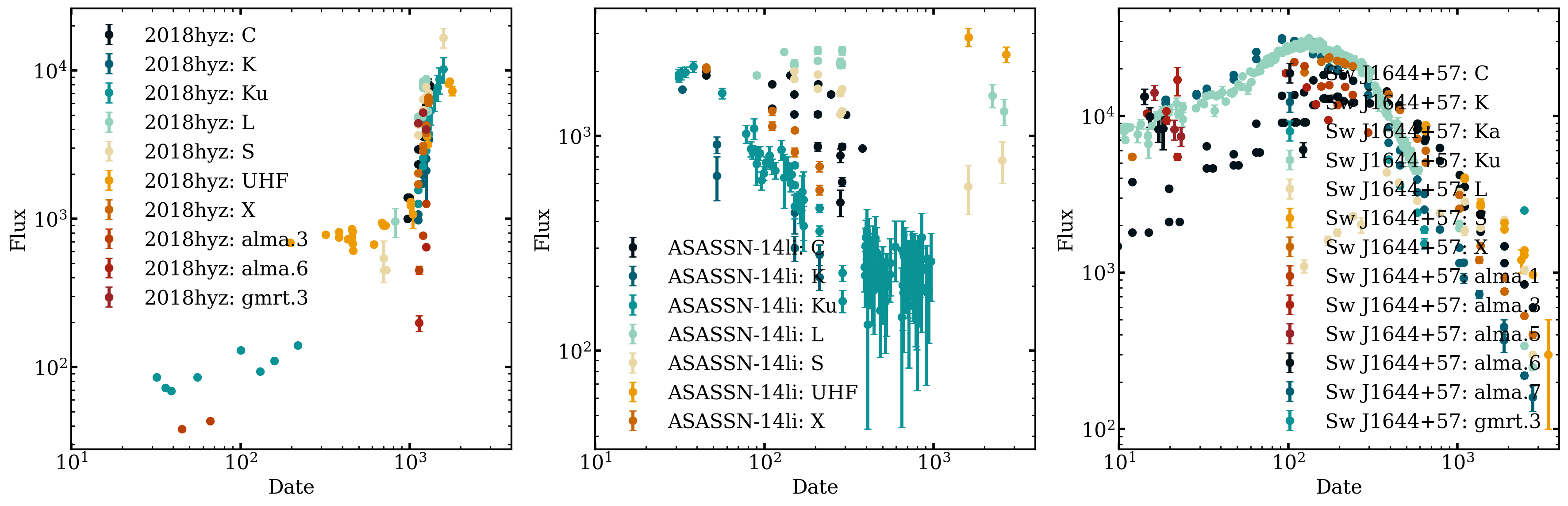
../_images/examples_basic_usage_30_0.png

Where the colors represent the observation frequency! Obviously these are not pubblication ready but they are at least a good way to easily visualize the data while working with it.