Working with the Transient Class#
This notebook will go through working with the methods of the transient class and how they will be useful. First we will setup the otter connection, if this doesn’t look familiar to you, you may want to return to the basic_usage.ipynb notebook!
Setup#
[1]:
# imports
import os
import io
import otter

import json
import requests # you may need to pip install requests

from astropy.coordinates import SkyCoord
from astropy import units as u
import pandas as pd

import matplotlib.pyplot as plt
[2]:
# connect to the dataset
db = otter.Otter()
Attempting to login to https://otter.idies.jhu.edu/api with the following credentials:
username: user-guest
password: test
The Transient Class#
For the detailed documentation for this class see https://astro-otter.readthedocs.io.
The particularly useful methods here are the getters which return what we have deemed to be the “default” value of a property.
First though, we must grab a transient from the OTTER dataset. Let’s use ASASSN-14li since it has a pretty solid dataset.
[3]:
t = db.query(names='ASASSN-14li')[0] # if you don't know why I use [0] go back to the basic_usage tutorial

t
[3]:
Transient(
        Name: ASASSN-14li,
        Keys: dict_keys(['_key', '_id', '_rev', '_dec', '_ra', 'classification', 'coordinate', 'date_reference', 'distance', 'filter_alias', 'host', 'name', 'photometry', 'reference_alias', 'schema_version'])
)
And now that next few cells will demonstrate some of the more helpful getter methods and instance variables
Name#
[4]:
t.default_name
[4]:
'ASASSN-14li'
Coordinate#
Note that this returns an astropy SkyCoord
[5]:
t.get_skycoord()
[5]:
<SkyCoord (ICRS): (ra, dec) in deg
    (192.06343875, 17.77402083)>
Classification#
This returns a tuple of (classification, our confidence, reference list)
[6]:
classification, conf, refs = t.get_classification()
print(f'{t.default_name} is classified as {classification} with a confidence of {conf}')
print(f'This has been confirmed by the following bibcodes:')
for b in refs:
    print(f'\t-{b}')
ASASSN-14li is classified as TDE with a confidence of 3.3
This has been confirmed by the following bibcodes:
        -2012PASP..124..668Y
        -2014ATel.6777....1J
        -2015Natur.526..542M
        -2016ApJ...819L..25A
        -2016ApJ...832L..10R
        -2016Sci...351...62V
        -2018MNRAS.475.4011B
        -2023PASP..135c4101G
        -2024ApJ...966..160G
        -2024MNRAS.527.2452M
        -ASAS-SN Supernovae
Redshift#
[7]:
t.get_redshift()
[7]:
0.0206
Discovery Date#
[8]:
t.get_discovery_date()
[8]:
<Time object: scale='utc' format='mjd' value=56983.0>
Photometry#
Since the Transient object only has the unconverted photometry we recommend you use the clean_photometry method to convert everything appropriately.
[9]:
t.clean_photometry()
/home/nfranz/research/astro-otter/otter/src/otter/io/transient.py:1072: UserWarning: Boolean Series key will be reindexed to match DataFrame index.
  for val_av, grp in subset[outdata.corr_av == True].groupby("val_av"):
ASASSN-14li has at least one photometry point where it is unclear if a host subtraction was performed. This can be especially detrimental for UV data. Please consider filtering out UV/Optical/IR or radio rows where the corr_host column is null/None/NaN.
[9]:
| converted_flux | converted_flux_err | converted_date | converted_wave | converted_freq | converted_flux_unit | converted_date_unit | converted_wave_unit | converted_freq_unit | reference | ... | corr_s | _standard_filter_name | date | _flux_err | instrument | max_dates | computed | corr_av | _norm_tele_name | raw_err | |
|---|---|---|---|---|---|---|---|---|---|---|---|---|---|---|---|---|---|---|---|---|---|
| 0 | 15.383650 | 0.050567 | 51505.660000 | 2.141375e+08 | 1.40000 | mag(AB) | MJD | nm | GHz | 2016Sci...351...62V | ... | False | 1.4GHz | 51505.66 | 0.140000 | NaN | NaN | NaN | False | first | 0.140000 |
| 1 | 16.115142 | 0.127528 | 59598.900000 | 1.810888e+08 | 1.65550 | mag(AB) | MJD | nm | GHz | 2024ApJ...974..241A | ... | False | 1655.5MHz | 59598.9 | 0.180000 | NaN | NaN | NaN | False | racs | 0.180000 |
| 2 | 15.251519 | 0.089545 | 58597.500000 | 3.377943e+08 | 0.88750 | mag(AB) | MJD | nm | GHz | 2024ApJ...974..241A | ... | False | 887.5MHz | 58597.5 | 0.280000 | NaN | NaN | NaN | False | racs | 0.280000 |
| 3 | 15.454005 | 0.077074 | 59664.700000 | 3.377943e+08 | 0.88750 | mag(AB) | MJD | nm | GHz | 2024ApJ...974..241A | ... | False | 887.5MHz | 59664.7 | 0.200000 | NaN | NaN | NaN | False | racs | 0.200000 |
| 4 | 15.931198 | 0.113634 | 59213.000000 | 2.192267e+08 | 1.36750 | mag(AB) | MJD | nm | GHz | 2024ApJ...974..241A | ... | False | 1367.5MHz | 59213.0 | 0.190000 | NaN | NaN | NaN | False | racs | 0.190000 |
| ... | ... | ... | ... | ... | ... | ... | ... | ... | ... | ... | ... | ... | ... | ... | ... | ... | ... | ... | ... | ... | ... |
| 1120 | 18.403497 | 0.241133 | 57129.401341 | 3.434775e+02 | 872815.35755 | mag(AB) | MJD | nm | GHz | [2015Natur.526..542M, 2024MNRAS.527.2452M] | ... | False | U | 57129.401341 | 0.000018 | NaN | 57130.401341 | NaN | True | NaN | 0.000018 |
| 1121 | 19.161506 | 0.540408 | 57132.557014 | 3.434775e+02 | 872815.35755 | mag(AB) | MJD | nm | GHz | [2015Natur.526..542M, 2024MNRAS.527.2452M] | ... | False | U | 57132.557014 | 0.000020 | NaN | 57133.557014 | NaN | True | NaN | 0.000020 |
| 1122 | 19.006763 | 0.414131 | 57136.560133 | 3.434775e+02 | 872815.35755 | mag(AB) | MJD | nm | GHz | [2015Natur.526..542M, 2024MNRAS.527.2452M] | ... | False | U | 57136.560133 | 0.000018 | NaN | 57137.560133 | NaN | True | NaN | 0.000018 |
| 1123 | 18.839023 | 0.329726 | 57139.349452 | 3.434775e+02 | 872815.35755 | mag(AB) | MJD | nm | GHz | [2015Natur.526..542M, 2024MNRAS.527.2452M] | ... | False | U | 57139.349452 | 0.000017 | NaN | 57140.349452 | NaN | True | NaN | 0.000017 |
| 1124 | 19.446421 | 0.556577 | 57147.598925 | 3.434775e+02 | 872815.35755 | mag(AB) | MJD | nm | GHz | [2015Natur.526..542M, 2024MNRAS.527.2452M] | ... | False | U | 57147.598925 | 0.000016 | NaN | 57148.598925 | NaN | True | NaN | 0.000016 |
1125 rows × 53 columns
Host Information#
This will return a list of otter Host objects. See the tutorial host_objects.ipynb for more details on the functionality we provide here.
The Host objects only store metadata on the host like redshift, ra, dec, and name. If a Host is not in OTTER, we attempt to find the best matching hosts using astro-ghost.
[10]:
hlist = t.get_host()
h0 = hlist[0]

h0, type(hlist), type(h0)
[10]:
(SDSS J124815.23+174626.4 @ (RA, Dec)=(192.06249999999997 deg,17.77401111111111 deg),
 list,
 otter.io.host.Host)
Advanced Usage of the Transient Class#
Say you want other information that is not easily accessible by the getters shown above. Or, you think we are wrong about the default value for that property. You can then just treat the Transient object like a python dictionary to access the other values for those properties yourself.
First, it has a keys method, so let’s start there.
[11]:
t.keys()
[11]:
dict_keys(['_key', '_id', '_rev', '_dec', '_ra', 'classification', 'coordinate', 'date_reference', 'distance', 'filter_alias', 'host', 'name', 'photometry', 'reference_alias', 'schema_version'])
Let’s say you want to see what other distance measurements exist for ASASSN-14li besides the redshift. Let’s check that property
[12]:
t['distance']
[12]:
[{'value': '0.019999999552965164',
  'distance_type': 'redshift',
  'reference': ['2024ApJ...966..160G'],
  'default': False},
 {'value': '0.0205778',
  'distance_type': 'redshift',
  'reference': ['2015Natur.526..542M', '2024MNRAS.527.2452M'],
  'default': False},
 {'value': '0.0206',
  'distance_type': 'redshift',
  'reference': ['2012PASP..124..668Y',
   '2014ATel.6777....1J',
   '2015arXiv150701598H',
   '2016ApJ...819L..25A',
   '2016ApJ...832L..10R',
   '2016Sci...351...62V',
   '2017ApJ...838..149A',
   '2018MNRAS.475.4011B',
   '2023PASP..135c4101G',
   'ASAS-SN Supernovae'],
  'default': True},
 {'value': '0.021',
  'distance_type': 'redshift',
  'reference': ['2024ApJ...974..241A'],
  'default': False},
 {'value': '81.0',
  'distance_type': 'dispersion_measure',
  'unit': 'km/s',
  'reference': ['2017MNRAS.471.1694W', '2024MNRAS.527.2452M'],
  'default': True},
 {'value': '90.7',
  'distance_type': 'comoving',
  'unit': 'Mpc',
  'reference': ['2012PASP..124..668Y',
   '2014ATel.6777....1J',
   '2015arXiv150701598H',
   '2016A&A...594A..13P',
   '2017ApJ...835...64G',
   '2017ApJ...838..149A',
   'ASAS-SN Supernovae'],
  'default': True},
 {'value': '92.6',
  'distance_type': 'luminosity',
  'unit': 'Mpc',
  'reference': ['2012PASP..124..668Y',
   '2014ATel.6777....1J',
   '2015arXiv150701598H',
   '2016A&A...594A..13P',
   '2017ApJ...835...64G',
   '2017ApJ...838..149A',
   'ASAS-SN Supernovae'],
  'default': True}]
Just like most of the properties here, it is a list of distances with some keywords that tell you about it.
To work with this, we can simply put it in a pandas dataframe and filter it accordingly. Say you only want luminosity distances, we can then filter that pandas dataframe by the distance_type column.
[13]:
dists = pd.DataFrame(t['distance'])
lum_dists = dists[dists.distance_type == 'luminosity']
lum_dists
[13]:
| value | distance_type | reference | default | unit | |
|---|---|---|---|---|---|
| 6 | 92.6 | luminosity | [2012PASP..124..668Y, 2014ATel.6777....1J, 201... | True | Mpc |
Which then gives you a luminosity distance and the references you need to cite when you put it in your paper!
A similar process can be used for the rest of the properties so I won’t go through them in detail here but just remember, the Transient objects are basically just fancy python dictionaries!
Querying WISeREP for spectra of this Transient#
As an example, let’s consider the TDE 2019azh. Downloading all the spectra from WISeREP will take a little bit, but it should be pretty easy with the OTTER API!
[14]:
t = db.get_meta(names="2019azh")[0]
spec = t.get_wiserep_spec()
spec
www.wiserep.org/system/files/uploaded/ePESSTO/AT2019azh_2019-02-25_03-48-04.048_ESO-NTT_EFOSC2-NTT_ePESSTO.fits
www.wiserep.org/system/files/uploaded/PESSTO_SSDR1-4/AT2019azh_2019-02-25_03-48-04_ESO-NTT_EFOSC2-NTT_PESSTO_SSDR1-4.fits
www.wiserep.org/system/files/uploaded/StarDestroyers/2019azh_2019-03-14_10-30-33.746_FTN_FLOYDS-N_StarDestroyers.fits
www.wiserep.org/system/files/uploaded/PESSTO_SSDR1-4/AT2019azh_2019-03-19_03-18-04_ESO-NTT_EFOSC2-NTT_PESSTO_SSDR1-4.fits
www.wiserep.org/system/files/uploaded/PESSTO_SSDR1-4/AT2019azh_2019-03-19_03-33-54_ESO-NTT_EFOSC2-NTT_PESSTO_SSDR1-4.fits
www.wiserep.org/system/files/uploaded/StarDestroyers/2019azh_2020-04-20_07-50-25.897_FTN_FLOYDS-N_StarDestroyers.fits
www.wiserep.org/system/files/uploaded/StarDestroyers/2019azh_2020-05-13_06-18-42.690_FTN_FLOYDS-N_StarDestroyers.fits
/home/nfranz/research/astro-otter/otter/src/otter/io/data_finder.py:632: ParserWarning: Length of header or names does not match length of data. This leads to a loss of data with index_col=False.
  tab = pd.read_csv(ascii_file, index_col=False)
/home/nfranz/research/astro-otter/otter/src/otter/io/data_finder.py:632: ParserWarning: Length of header or names does not match length of data. This leads to a loss of data with index_col=False.
  tab = pd.read_csv(ascii_file, index_col=False)
/home/nfranz/research/astro-otter/otter/src/otter/io/data_finder.py:632: ParserWarning: Length of header or names does not match length of data. This leads to a loss of data with index_col=False.
  tab = pd.read_csv(ascii_file, index_col=False)
[14]:
( Spec. ID Obj. ID Obj. IAU Name \
0 51181 11910 TDE 2019azh
1 71786 11910 TDE 2019azh
2 83965 11910 TDE 2019azh
3 83966 11910 TDE 2019azh
4 83967 11910 TDE 2019azh
5 83968 11910 TDE 2019azh
6 83970 11910 TDE 2019azh
7 83969 11910 TDE 2019azh
8 83971 11910 TDE 2019azh
9 83972 11910 TDE 2019azh
10 83973 11910 TDE 2019azh
11 83964 11910 TDE 2019azh
12 83974 11910 TDE 2019azh
13 57466 11910 TDE 2019azh
14 83975 11910 TDE 2019azh
15 71785 11910 TDE 2019azh
16 71784 11910 TDE 2019azh
17 83976 11910 TDE 2019azh
18 83977 11910 TDE 2019azh
19 83978 11910 TDE 2019azh
20 83979 11910 TDE 2019azh
21 83980 11910 TDE 2019azh
22 83981 11910 TDE 2019azh
23 83982 11910 TDE 2019azh
24 83983 11910 TDE 2019azh
25 83984 11910 TDE 2019azh
26 83985 11910 TDE 2019azh
27 83986 11910 TDE 2019azh
28 83987 11910 TDE 2019azh
29 83988 11910 TDE 2019azh
30 83989 11910 TDE 2019azh
31 83990 11910 TDE 2019azh
32 83991 11910 TDE 2019azh
33 83992 11910 TDE 2019azh
34 83993 11910 TDE 2019azh
35 83994 11910 TDE 2019azh
36 83995 11910 TDE 2019azh
37 83996 11910 TDE 2019azh
38 83997 11910 TDE 2019azh
39 83998 11910 TDE 2019azh
40 83999 11910 TDE 2019azh
Obj. Alt. Name/s Obj Family Type \
0 ZTF18achzddr, Gaia19bvo, ZTF17aaazdba, ASASSN-... Nuclear
1 ZTF18achzddr, Gaia19bvo, ZTF17aaazdba, ASASSN-... Nuclear
2 ZTF18achzddr, Gaia19bvo, ZTF17aaazdba, ASASSN-... Nuclear
3 ZTF18achzddr, Gaia19bvo, ZTF17aaazdba, ASASSN-... Nuclear
4 ZTF18achzddr, Gaia19bvo, ZTF17aaazdba, ASASSN-... Nuclear
5 ZTF18achzddr, Gaia19bvo, ZTF17aaazdba, ASASSN-... Nuclear
6 ZTF18achzddr, Gaia19bvo, ZTF17aaazdba, ASASSN-... Nuclear
7 ZTF18achzddr, Gaia19bvo, ZTF17aaazdba, ASASSN-... Nuclear
8 ZTF18achzddr, Gaia19bvo, ZTF17aaazdba, ASASSN-... Nuclear
9 ZTF18achzddr, Gaia19bvo, ZTF17aaazdba, ASASSN-... Nuclear
10 ZTF18achzddr, Gaia19bvo, ZTF17aaazdba, ASASSN-... Nuclear
11 ZTF18achzddr, Gaia19bvo, ZTF17aaazdba, ASASSN-... Nuclear
12 ZTF18achzddr, Gaia19bvo, ZTF17aaazdba, ASASSN-... Nuclear
13 ZTF18achzddr, Gaia19bvo, ZTF17aaazdba, ASASSN-... Nuclear
14 ZTF18achzddr, Gaia19bvo, ZTF17aaazdba, ASASSN-... Nuclear
15 ZTF18achzddr, Gaia19bvo, ZTF17aaazdba, ASASSN-... Nuclear
16 ZTF18achzddr, Gaia19bvo, ZTF17aaazdba, ASASSN-... Nuclear
17 ZTF18achzddr, Gaia19bvo, ZTF17aaazdba, ASASSN-... Nuclear
18 ZTF18achzddr, Gaia19bvo, ZTF17aaazdba, ASASSN-... Nuclear
19 ZTF18achzddr, Gaia19bvo, ZTF17aaazdba, ASASSN-... Nuclear
20 ZTF18achzddr, Gaia19bvo, ZTF17aaazdba, ASASSN-... Nuclear
21 ZTF18achzddr, Gaia19bvo, ZTF17aaazdba, ASASSN-... Nuclear
22 ZTF18achzddr, Gaia19bvo, ZTF17aaazdba, ASASSN-... Nuclear
23 ZTF18achzddr, Gaia19bvo, ZTF17aaazdba, ASASSN-... Nuclear
24 ZTF18achzddr, Gaia19bvo, ZTF17aaazdba, ASASSN-... Nuclear
25 ZTF18achzddr, Gaia19bvo, ZTF17aaazdba, ASASSN-... Nuclear
26 ZTF18achzddr, Gaia19bvo, ZTF17aaazdba, ASASSN-... Nuclear
27 ZTF18achzddr, Gaia19bvo, ZTF17aaazdba, ASASSN-... Nuclear
28 ZTF18achzddr, Gaia19bvo, ZTF17aaazdba, ASASSN-... Nuclear
29 ZTF18achzddr, Gaia19bvo, ZTF17aaazdba, ASASSN-... Nuclear
30 ZTF18achzddr, Gaia19bvo, ZTF17aaazdba, ASASSN-... Nuclear
31 ZTF18achzddr, Gaia19bvo, ZTF17aaazdba, ASASSN-... Nuclear
32 ZTF18achzddr, Gaia19bvo, ZTF17aaazdba, ASASSN-... Nuclear
33 ZTF18achzddr, Gaia19bvo, ZTF17aaazdba, ASASSN-... Nuclear
34 ZTF18achzddr, Gaia19bvo, ZTF17aaazdba, ASASSN-... Nuclear
35 ZTF18achzddr, Gaia19bvo, ZTF17aaazdba, ASASSN-... Nuclear
36 ZTF18achzddr, Gaia19bvo, ZTF17aaazdba, ASASSN-... Nuclear
37 ZTF18achzddr, Gaia19bvo, ZTF17aaazdba, ASASSN-... Nuclear
38 ZTF18achzddr, Gaia19bvo, ZTF17aaazdba, ASASSN-... Nuclear
39 ZTF18achzddr, Gaia19bvo, ZTF17aaazdba, ASASSN-... Nuclear
40 ZTF18achzddr, Gaia19bvo, ZTF17aaazdba, ASASSN-... Nuclear
Obj Type Redshift Obs-date (UT) Phase/s Tel / Inst \
0 TDE 0.022 2019-02-25 03:48:04.00 NaN ESO-NTT / EFOSC2-NTT
1 TDE 0.022 2019-02-25 03:48:04.00 NaN ESO-NTT / EFOSC2-NTT
2 TDE 0.022 2019-02-28 22:05:15.00 NaN Ekar / AFOSC
3 TDE 0.022 2019-03-01 20:33:34.00 NaN Ekar / AFOSC
4 TDE 0.022 2019-03-02 21:19:28.00 NaN Ekar / AFOSC
5 TDE 0.022 2019-03-03 00:00:00.00 NaN LCO-duPont / WFCCD
6 TDE 0.022 2019-03-05 00:00:00.00 NaN LCO-duPont / WFCCD
7 TDE 0.022 2019-03-05 20:20:04.00 NaN Ekar / AFOSC
8 TDE 0.022 2019-03-07 00:00:00.00 NaN LCO-duPont / WFCCD
9 TDE 0.022 2019-03-08 19:01:36.00 NaN Ekar / AFOSC
10 TDE 0.022 2019-03-13 10:02:43.00 NaN FTN / FLOYDS-N
11 TDE 0.022 2019-03-14 10:30:33.00 NaN FTN / FLOYDS-N
12 TDE 0.022 2019-03-14 21:06:09.00 NaN Ekar / AFOSC
13 TDE 0.022 2019-03-15 09:22:38.00 NaN P60 / SEDM
14 TDE 0.022 2019-03-17 00:00:00.00 NaN Lick-3m / KAST
15 TDE 0.022 2019-03-19 03:18:04.00 NaN ESO-NTT / EFOSC2-NTT
16 TDE 0.022 2019-03-19 03:33:54.00 NaN ESO-NTT / EFOSC2-NTT
17 TDE 0.022 2019-03-19 07:36:11.00 NaN FTN / FLOYDS-N
18 TDE 0.022 2019-03-24 07:09:30.00 NaN FTN / FLOYDS-N
19 TDE 0.022 2019-03-30 08:25:39.00 NaN FTN / FLOYDS-N
20 TDE 0.022 2019-03-31 00:00:00.00 NaN Lick-3m / KAST
21 TDE 0.022 2019-04-05 08:22:23.00 NaN FTN / FLOYDS-N
22 TDE 0.022 2019-04-07 07:27:57.00 NaN FTN / FLOYDS-N
23 TDE 0.022 2019-04-09 00:00:00.00 NaN LCO-duPont / WFCCD
24 TDE 0.022 2019-04-09 09:53:20.00 NaN FTN / FLOYDS-N
25 TDE 0.022 2019-04-16 05:51:40.00 NaN FTN / FLOYDS-N
26 TDE 0.022 2019-04-23 08:56:18.00 NaN FTN / FLOYDS-N
27 TDE 0.022 2019-04-25 00:00:00.00 NaN Lick-3m / KAST
28 TDE 0.022 2019-05-12 00:00:00.00 NaN Lick-3m / KAST
29 TDE 0.022 2019-06-05 00:00:00.00 NaN Lick-3m / KAST
30 TDE 0.022 2019-10-15 13:38:25.00 NaN FTN / FLOYDS-N
31 TDE 0.022 2019-12-03 16:15:15.00 NaN FTN / FLOYDS-N
32 TDE 0.022 2019-12-19 14:14:03.00 NaN FTN / FLOYDS-N
33 TDE 0.022 2020-01-18 11:38:12.00 NaN FTN / FLOYDS-N
34 TDE 0.022 2020-02-02 00:00:00.00 NaN WHT-4.2m / ISIS
35 TDE 0.022 2020-02-02 23:08:57.00 NaN WHT-4.2m / ISIS
36 TDE 0.022 2020-02-05 07:20:14.00 NaN FTN / FLOYDS-N
37 TDE 0.022 2020-02-28 11:08:22.00 NaN FTN / FLOYDS-N
38 TDE 0.022 2020-03-22 09:23:23.00 NaN FTN / FLOYDS-N
39 TDE 0.022 2020-04-20 07:50:25.00 NaN FTN / FLOYDS-N
40 TDE 0.022 2020-05-13 06:18:42.00 NaN FTN / FLOYDS-N
... Public End Prop. Period Reporter/s Publish Contrib \
0 ... Y NaN NaN NaN NaN
1 ... Y NaN NaN NaN NaN
2 ... Y NaN NaN NaN NaN
3 ... Y NaN NaN NaN NaN
4 ... Y NaN NaN NaN NaN
5 ... Y NaN NaN NaN NaN
6 ... Y NaN NaN NaN NaN
7 ... Y NaN NaN NaN NaN
8 ... Y NaN NaN NaN NaN
9 ... Y NaN NaN NaN NaN
10 ... Y NaN NaN NaN NaN
11 ... Y NaN NaN NaN NaN
12 ... Y NaN NaN NaN NaN
13 ... Y NaN NaN NaN NaN
14 ... Y NaN NaN NaN NaN
15 ... Y NaN NaN NaN NaN
16 ... Y NaN NaN NaN NaN
17 ... Y NaN NaN NaN NaN
18 ... Y NaN NaN NaN NaN
19 ... Y NaN NaN NaN NaN
20 ... Y NaN NaN NaN NaN
21 ... Y NaN NaN NaN NaN
22 ... Y NaN NaN NaN NaN
23 ... Y NaN NaN NaN NaN
24 ... Y NaN NaN NaN NaN
25 ... Y NaN NaN NaN NaN
26 ... Y NaN NaN NaN NaN
27 ... Y NaN NaN NaN NaN
28 ... Y NaN NaN NaN NaN
29 ... Y NaN NaN NaN NaN
30 ... Y NaN NaN NaN NaN
31 ... Y NaN NaN NaN NaN
32 ... Y NaN NaN NaN NaN
33 ... Y NaN NaN NaN NaN
34 ... Y NaN NaN NaN NaN
35 ... Y NaN NaN NaN NaN
36 ... Y NaN NaN NaN NaN
37 ... Y NaN NaN NaN NaN
38 ... Y NaN NaN NaN NaN
39 ... Y NaN NaN NaN NaN
40 ... Y NaN NaN NaN NaN
Remarks Created by Creation date (UT) \
0 NaN WIS_Bot1 2019-02-25 12:19:59
1 Released as part of DR4 WIS_Bot1 2023-05-04 13:51:10
2 NaN Ms Sara Faris 2024-10-25 16:33:24
3 NaN Ms Sara Faris 2024-10-25 16:39:04
4 NaN Ms Sara Faris 2024-10-25 16:39:04
5 NaN Ms Sara Faris 2024-10-25 16:53:49
6 NaN Ms Sara Faris 2024-10-25 17:36:35
7 NaN Ms Sara Faris 2024-10-25 17:36:35
8 NaN Ms Sara Faris 2024-10-25 17:44:53
9 NaN Ms Sara Faris 2024-10-25 17:44:53
10 NaN Ms Sara Faris 2024-10-25 17:44:53
11 NaN Ms Sara Faris 2024-10-25 15:27:18
12 NaN Ms Sara Faris 2024-10-25 18:08:25
13 [TNS source group: 48 - ZTF ] TNS_Bot1 2020-07-13 17:05:05
14 NaN Ms Sara Faris 2024-10-25 18:08:25
15 Released as part of DR4 WIS_Bot1 2023-05-04 13:51:10
16 Released as part of DR4 WIS_Bot1 2023-05-04 13:51:10
17 NaN Ms Sara Faris 2024-10-25 18:15:10
18 NaN Ms Sara Faris 2024-10-25 18:15:10
19 NaN Ms Sara Faris 2024-10-25 18:15:10
20 NaN Ms Sara Faris 2024-10-26 08:32:27
21 NaN Ms Sara Faris 2024-10-26 08:32:27
22 NaN Ms Sara Faris 2024-10-26 08:32:27
23 NaN Ms Sara Faris 2024-10-26 08:32:27
24 NaN Ms Sara Faris 2024-10-26 08:32:27
25 NaN Ms Sara Faris 2024-10-26 08:48:31
26 NaN Ms Sara Faris 2024-10-26 08:48:31
27 NaN Ms Sara Faris 2024-10-26 08:48:31
28 NaN Ms Sara Faris 2024-10-26 08:48:31
29 NaN Ms Sara Faris 2024-10-26 08:48:31
30 NaN Ms Sara Faris 2024-10-26 08:48:31
31 NaN Ms Sara Faris 2024-10-26 08:48:31
32 NaN Ms Sara Faris 2024-10-26 08:55:23
33 NaN Ms Sara Faris 2024-10-26 08:55:23
34 NaN Ms Sara Faris 2024-10-26 08:55:23
35 NaN Ms Sara Faris 2024-10-26 09:01:02
36 NaN Ms Sara Faris 2024-10-26 09:01:02
37 NaN Ms Sara Faris 2024-10-26 09:01:02
38 NaN Ms Sara Faris 2024-10-26 09:01:02
39 NaN Ms Sara Faris 2024-10-26 09:03:59
40 NaN Ms Sara Faris 2024-10-26 09:03:59
Modified by Last modified date (UT)
0 WIS_Bot1 2022-09-18 15:05:17
1 WIS_Bot1 2023-05-04 14:20:44
2 Ms Sara Faris 2024-10-25 17:47:01
3 Ms Sara Faris 2024-10-25 17:36:57
4 Ms Sara Faris 2024-10-25 17:37:40
5 Ms Sara Faris 2024-10-26 08:33:52
6 Ms Sara Faris 2024-10-26 08:33:40
7 Ms Sara Faris 2024-10-25 17:50:42
8 Ms Sara Faris 2024-10-26 08:33:26
9 Ms Sara Faris 2024-10-25 17:53:02
10 Ms Sara Faris 2024-10-25 17:44:53
11 Ms Sara Faris 2024-10-25 15:27:18
12 Ms Sara Faris 2024-10-25 18:08:25
13 TNS_Bot1 2022-09-18 15:05:17
14 Ms Sara Faris 2024-10-25 18:08:25
15 WIS_Bot1 2023-05-04 14:20:44
16 WIS_Bot1 2023-05-04 14:20:44
17 Ms Sara Faris 2024-10-25 18:15:10
18 Ms Sara Faris 2024-10-25 18:15:10
19 Ms Sara Faris 2024-10-25 18:15:10
20 Ms Sara Faris 2024-10-26 08:32:27
21 Ms Sara Faris 2024-10-26 08:32:27
22 Ms Sara Faris 2024-10-26 08:32:27
23 Ms Sara Faris 2024-10-26 08:32:27
24 Ms Sara Faris 2024-10-26 08:32:27
25 Ms Sara Faris 2024-10-26 08:48:31
26 Ms Sara Faris 2024-10-26 08:48:31
27 Ms Sara Faris 2024-10-26 08:48:31
28 Ms Sara Faris 2024-10-26 08:48:31
29 Ms Sara Faris 2024-10-26 08:48:31
30 Ms Sara Faris 2024-10-26 08:48:31
31 Ms Sara Faris 2024-10-26 08:48:31
32 Ms Sara Faris 2024-10-26 08:55:23
33 Ms Sara Faris 2024-10-26 08:55:23
34 Ms Sara Faris 2024-10-26 08:56:21
35 Ms Sara Faris 2024-10-26 09:01:02
36 Ms Sara Faris 2024-10-26 09:01:02
37 Ms Sara Faris 2024-10-26 09:01:02
38 Ms Sara Faris 2024-10-26 09:01:02
39 Ms Sara Faris 2024-10-26 09:03:59
40 Ms Sara Faris 2024-10-26 09:03:59
[41 rows x 33 columns],
{0: wave flux
0 3634.047852 5.716230e-15
1 3639.565780 5.764000e-15
2 3645.083709 5.788830e-15
3 3650.601637 5.839910e-15
4 3656.119566 5.866310e-15
... ... ...
1010 9207.155738 6.875600e-16
1011 9212.673666 6.513190e-16
1012 9218.191595 7.254140e-16
1013 9223.709524 7.590670e-16
1014 9229.227452 7.131390e-16
[1015 rows x 2 columns],
1: wave flux
0 3633.3237 6.067978e-15
1 3638.8433 6.058791e-15
2 3644.3630 6.077160e-15
3 3649.8828 6.085601e-15
4 3655.4023 5.986992e-15
... ... ...
1010 9208.2110 1.028024e-15
1011 9213.7310 1.031048e-15
1012 9219.2510 1.063123e-15
1013 9224.7705 1.088238e-15
1014 9230.2900 1.047404e-15
[1015 rows x 2 columns],
2: wave flux
0 3181.035890 1.134581e-14
1 3184.992053 1.199393e-14
2 3188.948215 1.166145e-14
3 3192.904377 1.090576e-14
4 3196.860540 1.139100e-14
... ... ...
1489 9071.761633 1.505913e-16
1490 9075.717795 1.451773e-16
1491 9079.673957 1.404678e-16
1492 9083.630120 1.361425e-16
1493 9087.586282 1.317531e-16
[1494 rows x 2 columns],
3: wave flux
0 3200.525950 1.186926e-14
1 3204.481651 1.150676e-14
2 3208.437352 1.116650e-14
3 3212.393053 1.089178e-14
4 3216.348754 1.085625e-14
... ... ...
1484 9070.786138 1.010047e-16
1485 9074.741839 9.725177e-17
1486 9078.697540 9.355036e-17
1487 9082.653241 9.027793e-17
1488 9086.608942 8.694844e-17
[1489 rows x 2 columns],
4: wave flux
0 3140.781863 1.523502e-14
1 3144.737770 1.254093e-14
2 3148.693677 1.107019e-14
3 3152.649585 1.289846e-14
4 3156.605492 1.276622e-14
... ... ...
1499 9070.686502 1.299114e-16
1500 9074.642409 1.255178e-16
1501 9078.598316 1.200511e-16
1502 9082.554223 1.156804e-16
1503 9086.510130 1.118889e-16
[1504 rows x 2 columns],
5: wave flux
0 4201.0 4.305530e-15
1 4202.0 4.247704e-15
2 4204.0 4.110278e-15
3 4206.0 4.027790e-15
4 4208.0 3.893335e-15
... ... ...
1971 7990.0 1.583881e-15
1972 7992.0 1.576428e-15
1973 7994.0 1.571701e-15
1974 7996.0 1.576368e-15
1975 7998.0 1.566160e-15
[1976 rows x 2 columns],
6: wave flux
0 4202.0 4.456432e-15
1 4204.0 4.363146e-15
2 4205.0 4.235708e-15
3 4207.0 4.086436e-15
4 4209.0 3.841205e-15
... ... ...
1970 7991.0 1.160506e-15
1971 7993.0 1.157680e-15
1972 7995.0 1.147042e-15
1973 7997.0 1.159000e-15
1974 7999.0 1.144324e-15
[1975 rows x 2 columns],
7: wave flux
0 3144.151547 1.364624e-14
1 3148.107323 1.227980e-14
2 3152.063100 1.335542e-14
3 3156.018876 1.353157e-14
4 3159.974653 1.272943e-14
... ... ...
1498 9069.904866 -2.142106e-17
1499 9073.860642 -2.197199e-17
1500 9077.816419 -2.245656e-17
1501 9081.772195 -2.287409e-17
1502 9085.727972 -2.320858e-17
[1503 rows x 2 columns],
8: wave flux
0 4202.0 4.543918e-15
1 4204.0 4.423192e-15
2 4206.0 4.306467e-15
3 4207.0 4.069442e-15
4 4209.0 4.050455e-15
... ... ...
1971 7990.0 1.691671e-15
1972 7992.0 1.677981e-15
1973 7994.0 1.702301e-15
1974 7996.0 1.705288e-15
1975 7998.0 1.716856e-15
[1976 rows x 2 columns],
9: wave flux
0 3274.146380 1.076063e-14
1 3278.104553 1.013153e-14
2 3282.062726 9.864911e-15
3 3286.020900 9.434134e-15
4 3289.979073 9.238699e-15
... ... ...
1464 9068.912222 -1.963720e-16
1465 9072.870395 -1.911188e-16
1466 9076.828569 -1.863280e-16
1467 9080.786742 -1.809328e-16
1468 9084.744915 -1.750478e-16
[1469 rows x 2 columns],
10: wave flux
0 3426.597264 7.267902e-15
1 3428.300591 7.195238e-15
2 3430.003917 7.195882e-15
3 3431.707244 7.134539e-15
4 3433.410570 7.086520e-15
... ... ...
3151 8793.779203 3.100471e-16
3152 8795.482530 3.071652e-16
3153 8797.185856 3.082952e-16
3154 8798.889183 3.092468e-16
3155 8800.592509 3.071669e-16
[3156 rows x 2 columns],
11: wave flux
0 3499.291016 6.616641e-15
1 3501.032285 6.632436e-15
2 3502.773555 6.666119e-15
3 3504.514824 6.525637e-15
4 3506.256094 6.409819e-15
... ... ...
3729 9992.485311 1.016803e-15
3730 9994.226581 9.807904e-16
3731 9995.967850 9.446050e-16
3732 9997.709120 9.397874e-16
3733 9999.450389 9.919220e-16
[3734 rows x 2 columns],
12: wave flux
0 3334.105423 9.765602e-15
1 3338.697998 9.777363e-15
2 3343.290574 9.870621e-15
3 3347.883149 9.576106e-15
4 3352.475725 9.511858e-15
... ... ...
1014 7990.976969 9.243429e-16
1015 7995.569544 9.143546e-16
1016 8000.162120 9.093112e-16
1017 8004.754695 9.090894e-16
1018 8009.347271 9.074550e-16
[1019 rows x 2 columns],
13: wave flux
0 3776.7 3.883000e-14
1 3802.3 3.797000e-14
2 3827.9 4.084000e-14
3 3853.4 4.214000e-14
4 3879.0 3.710000e-14
.. ... ...
209 9121.0 7.798000e-15
210 9146.6 7.987000e-15
211 9172.1 7.543000e-15
212 9197.7 6.740000e-15
213 9223.3 6.943000e-15
[214 rows x 2 columns],
14: wave flux
0 3626.0 4.138010
1 3628.0 4.342990
2 3630.0 4.780910
3 3632.0 4.285670
4 3634.0 4.297110
... ... ...
3523 10672.0 1.163460
3524 10674.0 1.055570
3525 10676.0 0.947671
3526 10678.0 0.322510
3527 10680.0 0.439916
[3528 rows x 2 columns],
15: wave flux
0 3334.5664 1.220751e-14
1 3338.6455 1.174571e-14
2 3342.7249 1.121568e-14
3 3346.8040 1.091139e-14
4 3350.8830 1.092654e-14
... ... ...
1006 7438.2114 1.965350e-15
1007 7442.2905 1.937911e-15
1008 7446.3696 1.990556e-15
1009 7450.4490 2.021318e-15
1010 7454.5283 1.958683e-15
[1011 rows x 2 columns],
16: wave flux
0 5990.1020 0.000000e+00
1 5994.3154 3.370222e-15
2 5998.5293 3.213288e-15
3 6002.7427 3.191193e-15
4 6006.9560 3.152140e-15
.. ... ...
945 9971.9170 8.881983e-16
946 9976.1300 8.880565e-16
947 9980.3440 8.741274e-16
948 9984.5580 8.928276e-16
949 9988.7705 9.064272e-16
[950 rows x 2 columns],
17: wave flux
0 3427.667972 8.059685e-15
1 3429.371426 8.076899e-15
2 3431.074881 8.092160e-15
3 3432.778335 8.101097e-15
4 3434.481789 8.035194e-15
... ... ...
3725 9773.035018 2.789172e-16
3726 9774.738472 2.739608e-16
3727 9776.441926 2.720988e-16
3728 9778.145380 2.722470e-16
3729 9779.848835 2.704901e-16
[3730 rows x 2 columns],
18: wave flux
0 3428.153570 8.837629e-15
1 3429.857168 8.794304e-15
2 3431.560766 8.807359e-15
3 3433.264365 8.856871e-15
4 3434.967963 8.925227e-15
... ... ...
3724 9772.353070 3.369219e-16
3725 9774.056668 3.126785e-16
3726 9775.760266 2.941689e-16
3727 9777.463864 2.838706e-16
3728 9779.167462 2.827427e-16
[3729 rows x 2 columns],
19: wave flux
0 3428.126439 7.043469e-15
1 3429.829965 6.963396e-15
2 3431.533492 6.887640e-15
3 3433.237018 6.842861e-15
4 3434.940545 6.849194e-15
... ... ...
3294 9039.542873 5.342432e-16
3295 9041.246400 5.320611e-16
3296 9042.949926 5.280522e-16
3297 9044.653453 5.239494e-16
3298 9046.356979 5.208246e-16
[3299 rows x 2 columns],
20: wave flux
0 3612.0 10.91060
1 3614.0 10.91940
2 3616.0 10.94170
3 3618.0 10.76470
4 3620.0 11.24230
... ... ...
3541 10694.0 1.44293
3542 10696.0 1.58753
3543 10698.0 1.77105
3544 10700.0 1.81420
3545 10702.0 1.76955
[3546 rows x 2 columns],
21: wave flux
0 3427.998101 6.271847e-15
1 3429.701824 6.248290e-15
2 3431.405547 6.256379e-15
3 3433.109271 6.252506e-15
4 3434.812994 6.237170e-15
... ... ...
3724 9772.663589 2.643844e-16
3725 9774.367312 2.637155e-16
3726 9776.071035 2.624730e-16
3727 9777.774759 2.620241e-16
3728 9779.478482 2.612260e-16
[3729 rows x 2 columns],
22: wave flux
0 3427.619222 6.739359e-15
1 3429.322900 6.692292e-15
2 3431.026579 6.660125e-15
3 3432.730258 6.638945e-15
4 3434.433937 6.616953e-15
... ... ...
3724 9772.119247 2.077602e-16
3725 9773.822926 2.074212e-16
3726 9775.526605 2.090337e-16
3727 9777.230283 2.138813e-16
3728 9778.933962 2.211445e-16
[3729 rows x 2 columns],
23: wave flux
0 4202.0 4.603476e-15
1 4203.0 4.500239e-15
2 4205.0 4.513196e-15
3 4207.0 4.536475e-15
4 4208.0 4.609779e-15
... ... ...
1971 7991.0 1.149824e-15
1972 7993.0 1.140667e-15
1973 7995.0 1.142540e-15
1974 7997.0 1.119187e-15
1975 7999.0 1.122489e-15
[1976 rows x 2 columns],
24: wave flux
0 3721.001576 6.529429e-15
1 3722.703674 6.713370e-15
2 3724.405773 6.730355e-15
3 3726.107872 6.775230e-15
4 3727.809970 6.939945e-15
... ... ...
3555 9771.961942 1.119538e-16
3556 9773.664040 1.165707e-16
3557 9775.366139 1.195704e-16
3558 9777.068237 1.278590e-16
3559 9778.770336 1.387542e-16
[3560 rows x 2 columns],
25: wave flux
0 3428.147068 5.305901e-15
1 3429.850758 5.310080e-15
2 3431.554449 5.300657e-15
3 3433.258139 5.257551e-15
4 3434.961830 5.202080e-15
... ... ...
3724 9772.690521 2.341382e-16
3725 9774.394212 2.373442e-16
3726 9776.097902 2.375372e-16
3727 9777.801593 2.357688e-16
3728 9779.505283 2.336343e-16
[3729 rows x 2 columns],
26: wave flux
0 3426.675926 5.112305e-15
1 3428.378101 4.869209e-15
2 3430.080276 4.960809e-15
3 3431.782451 5.208071e-15
4 3433.484627 5.219276e-15
... ... ...
3697 9772.384974 1.027751e-16
3698 9774.087149 7.038761e-17
3699 9775.789324 4.340749e-17
3700 9777.491499 3.604578e-17
3701 9779.193674 3.995103e-17
[3702 rows x 2 columns],
27: wave flux
0 3614.0 4.860880
1 3616.0 4.778790
2 3618.0 4.862090
3 3620.0 4.816080
4 3622.0 4.623310
... ... ...
3529 10672.0 0.973877
3530 10674.0 0.876257
3531 10676.0 1.015720
3532 10678.0 0.971185
3533 10680.0 0.926649
[3534 rows x 2 columns],
28: wave flux
0 3616.0 4.107360
1 3618.0 3.915910
2 3620.0 3.949160
3 3622.0 4.039320
4 3624.0 4.057140
... ... ...
3545 10706.0 0.915080
3546 10708.0 0.924793
3547 10710.0 0.792116
3548 10712.0 0.938548
3549 10714.0 0.933729
[3550 rows x 2 columns],
29: wave flux
0 3612.0 1.380260
1 3614.0 1.248150
2 3616.0 1.473400
3 3618.0 1.399870
4 3620.0 1.140660
... ... ...
3591 10794.0 0.523627
3592 10796.0 0.512243
3593 10798.0 0.500859
3594 10800.0 0.403699
3595 10802.0 0.458975
[3596 rows x 2 columns],
30: wave flux
0 3428.841494 1.306619e-15
1 3431.079524 1.298456e-15
2 3433.317554 1.264040e-15
3 3435.555584 1.273227e-15
4 3437.793614 1.298002e-15
... ... ...
2833 9769.180592 -3.742782e-17
2834 9771.418622 -3.717722e-17
2835 9773.656652 -3.793955e-17
2836 9775.894682 -3.924759e-17
2837 9778.132712 -4.098766e-17
[2838 rows x 2 columns],
31: wave flux
0 3428.523711 1.242723e-15
1 3430.761794 1.214378e-15
2 3432.999876 1.184043e-15
3 3435.237959 1.222780e-15
4 3437.476041 1.273885e-15
... ... ...
2833 9769.011480 1.635686e-17
2834 9771.249563 1.718649e-17
2835 9773.487645 1.814483e-17
2836 9775.725728 1.893886e-17
2837 9777.963810 1.965327e-17
[2838 rows x 2 columns],
32: wave flux
0 3427.782121 1.050161e-15
1 3430.020198 1.073134e-15
2 3432.258274 1.085582e-15
3 3434.496351 1.102806e-15
4 3436.734428 1.128546e-15
... ... ...
2833 9768.253371 -1.112627e-16
2834 9770.491447 -1.109022e-16
2835 9772.729524 -1.123515e-16
2836 9774.967601 -1.144895e-16
2837 9777.205677 -1.148930e-16
[2838 rows x 2 columns],
33: wave flux
0 3428.859847 1.057303e-15
1 3431.098217 1.083032e-15
2 3433.336586 1.105919e-15
3 3435.574956 1.129586e-15
4 3437.813326 1.148654e-15
... ... ...
2833 9770.161009 -2.570771e-17
2834 9772.399378 -2.648173e-17
2835 9774.637748 -2.742069e-17
2836 9776.876117 -2.790889e-17
2837 9779.114487 -2.778696e-17
[2838 rows x 2 columns],
34: wave flux
0 3544.941299 1.493338e-15
1 3545.780975 1.485733e-15
2 3546.620650 1.540055e-15
3 3547.460325 1.586313e-15
4 3548.300001 1.627836e-15
... ... ...
1844 5093.302594 1.361655e-15
1845 5094.142270 1.359723e-15
1846 5094.981945 1.372850e-15
1847 5095.821620 1.378001e-15
1848 5096.661296 1.284680e-15
[1849 rows x 2 columns],
35: wave flux
0 5694.350280 1.200896e-15
1 5695.292483 1.092320e-15
2 5696.234686 1.077778e-15
3 5697.176888 1.079426e-15
4 5698.119091 1.081088e-15
... ... ...
1802 7392.199632 8.819493e-17
1803 7393.141835 7.537540e-17
1804 7394.084037 5.523331e-17
1805 7395.026240 3.634482e-17
1806 7395.968443 1.969845e-17
[1807 rows x 2 columns],
36: wave flux
0 3721.637259 1.673062e-15
1 3723.875970 1.612336e-15
2 3726.114682 1.577384e-15
3 3728.353393 1.552605e-15
4 3730.592105 1.448847e-15
... ... ...
2695 9768.397166 -2.904945e-17
2696 9770.635877 -2.784562e-17
2697 9772.874589 -2.681014e-17
2698 9775.113300 -2.603825e-17
2699 9777.352012 -2.645628e-17
[2700 rows x 2 columns],
37: wave flux
0 3427.757539 9.275095e-16
1 3429.995625 9.456181e-16
2 3432.233711 9.776202e-16
3 3434.471797 9.861508e-16
4 3436.709882 1.017078e-15
... ... ...
2833 9768.254559 -2.308410e-16
2834 9770.492644 -2.272570e-16
2835 9772.730730 -2.243294e-16
2836 9774.968816 -2.220540e-16
2837 9777.206902 -2.199870e-16
[2838 rows x 2 columns],
38: wave flux
0 3428.145408 1.149031e-15
1 3429.848866 1.146703e-15
2 3431.552323 1.126816e-15
3 3433.255781 1.129119e-15
4 3434.959239 1.120850e-15
... ... ...
3724 9771.822028 -1.048615e-16
3725 9773.525485 -1.041427e-16
3726 9775.228943 -1.042092e-16
3727 9776.932401 -1.048692e-16
3728 9778.635859 -1.055625e-16
[3729 rows x 2 columns],
39: wave flux
0 3500.389893 6.673363e-16
1 3502.077196 6.612603e-16
2 3503.764500 6.423367e-16
3 3505.451803 6.039406e-16
4 3507.139107 5.990139e-16
... ... ...
3848 9993.133926 1.017038e-15
3849 9994.821230 1.019430e-15
3850 9996.508533 9.573054e-16
3851 9998.195837 9.130978e-16
3852 9999.883141 9.149635e-16
[3853 rows x 2 columns],
40: wave flux
0 3500.836182 5.283473e-16
1 3502.577490 5.728877e-16
2 3504.318799 5.656475e-16
3 3506.060107 5.523856e-16
4 3507.801416 5.699351e-16
... ... ...
3728 9992.434530 4.560128e-16
3729 9994.175839 4.600028e-16
3730 9995.917147 4.595102e-16
3731 9997.658456 4.549676e-16
3732 9999.399765 4.555120e-16
[3733 rows x 2 columns]})
And so we just got a bunch of spectra from WISeREP on this object! In the OTTER API, we try to read in and standardize the spectra into a tuple (metadata, dictionary) for you. The keys in the spec[1] dictionary correspond to rows in the metadata dataframe.
[15]:
type(spec[0]), type(spec[1])
[15]:
(pandas.DataFrame, dict)
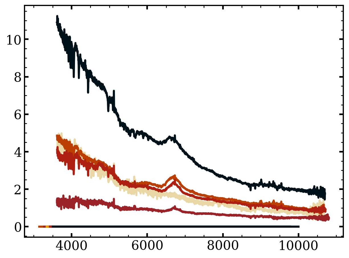
So we can now plot these spectra
[16]:
fig, ax = plt.subplots()
for k,s in spec[1].items():
    ax.plot(s.wave, s.flux)
[ ]: