Interfacing with Private Data

One of the main goals of OTTER is to make it easy to compare private data with the OTTER catalog, essentially interfacing with the OTTER dataset and private data together but without making your private data public!

Setup

%load_ext autoreload
%autoreload 2

import os
import pandas as pd
import matplotlib.pyplot as plt
import otter

Let’s say you’ve recently gotten two new observations of the TDE 2018hyz with the Very Large Array. You’ve reduced the data and extracted it and you’re curious how it looks compared to the previous radio observations of TDE 2018hyz. I’ve generated a fake dataset stored in the CSV format that OTTER expects (for both upload and interfacing with private data). Let’s start by reading those in and displaying them. Note that the required columns for the metadata are:

"name"
"ra"
"dec"
"ra_unit"
"dec_unit"
"coord_bibcode"

and the required columns for the photometry are:

"name"
"date"
"date_format"
"filter"
"filter_eff"
"filter_eff_units",
"flux"
"flux_err"
"flux_unit"

And then there are a bunch of optional columns, as listed on the upload page of the OTTER website. Note that these two tables will be merged based on the “name” column, so make sure those match appropriately.

meta = pd.read_csv("sample_meta.csv")
meta

	name	ra	dec	ra_unit	dec_unit	coord_bibcode	redshift	redshift_bibcode	discovery_date	discovery_date_format	discovery_date_bibcode	classification	classification_bibcode
0	2018hyz	10:06:50.87	01:41:34.08	hour	deg	2018TNSTR1708....1B	0.04573	2018TNSCR1764....1A	2018-11-06 15:21:36.000	iso	2018TNSTR1708....1B	TDE	2018TNSCR1764....1A

phot = pd.read_csv("sample_phot.csv")
phot

	name	flux	flux_unit	flux_err	date	date_format	filter	filter_eff	filter_eff_units
0	2018hyz	1	mJy	0.01	2025-05-20	iso	L	1.5	GHz
1	2018hyz	10	mJy	0.01	2025-05-23	iso	L	1.5	GHz

Combining this with the OTTER dataset

To combine this with the otter dataset, we use the Otter.from_csvs static method

# Connect to the otter database normally
db = otter.Otter()

# then use the Otter.from_csvs static method to read in the csvs simultaneously and tell otter where they are stored
db = otter.Otter.from_csvs(
    metafile = "sample_meta.csv",
    photfile = "sample_phot.csv",
    local_outpath = os.path.join(os.getcwd(), "private_otter_data"),
    db = db
)

print()
print(f"Your private data is stored in {db.DATADIR}")

Note the above warning, which shows that since we didn’t provide a bibcode for the photometry, it assumes that it is private and uses a special keyword for the bibcodes. However, you will have to add a bibcode column to the photometry csv file before uploading to OTTER.

Now that the Otter class (e.g. db in this notebook) knows about your private dataset, we can query otter almost exactly the same as normal. The only caveat is that we have to add query_private=True whenever we pass a query to the API.

As an example, let’s request all of the radio photometry.

allphot = db.get_phot(
    names="2018hyz",
    obs_type="radio",
    flux_unit="mJy",
    query_private=True,
    return_type="pandas"
)
allphot[allphot.reference == 'private']

Unable to apply the source mapping because 'private'

	name	converted_flux	converted_flux_err	converted_date	converted_wave	converted_freq	converted_flux_unit	converted_date_unit	converted_wave_unit	converted_freq_unit	filter_name	obs_type	upperlimit	reference	human_readable_refs	telescope
838	2018hyz	1.0	0.01	60815.0	1.998616e+08	1.5	mJy	MJD	nm	GHz	L	radio	False	private	private	NaN
839	2018hyz	10.0	0.01	60818.0	1.998616e+08	1.5	mJy	MJD	nm	GHz	L	radio	False	private	private	NaN

And, you can see that your private data is now accessible via the normal otter API!

Let’s plot up all of the L-band data for 18hyz

allphot[allphot.filter_name == "L"]

	name	converted_flux	converted_flux_err	converted_date	converted_wave	converted_freq	converted_flux_unit	converted_date_unit	converted_wave_unit	converted_freq_unit	filter_name	obs_type	upperlimit	reference	human_readable_refs	telescope
756	2018hyz	5.325	0.041	59686.00	2.306096e+08	1.3000	mJy	MJD	nm	GHz	L	radio	False	2022ApJ...938...28C	2022ApJ...938...28C	MeerKAT
793	2018hyz	4.850	0.220	59586.84	1.810888e+08	1.6555	mJy	MJD	nm	GHz	L	radio	False	2024ApJ...974..241A	2024ApJ...974..241A	RACS.high
812	2018hyz	0.960	0.210	59223.84	2.192267e+08	1.3675	mJy	MJD	nm	GHz	L	radio	False	2024ApJ...974..241A	2024ApJ...974..241A	RACS.mid
764	2018hyz	4.753	0.084	59530.00	2.188266e+08	1.3700	mJy	MJD	nm	GHz	L	radio	False	2022ApJ...938...28C	2022ApJ...938...28C	VLA
765	2018hyz	8.416	0.119	59603.00	2.188266e+08	1.3700	mJy	MJD	nm	GHz	L	radio	False	2022ApJ...938...28C	2022ApJ...938...28C	VLA
766	2018hyz	8.740	0.093	59655.00	2.188266e+08	1.3700	mJy	MJD	nm	GHz	L	radio	False	2022ApJ...938...28C	2022ApJ...938...28C	VLA
767	2018hyz	4.896	0.072	59530.00	1.850571e+08	1.6200	mJy	MJD	nm	GHz	L	radio	False	2022ApJ...938...28C	2022ApJ...938...28C	VLA
768	2018hyz	8.416	0.119	59603.00	1.850571e+08	1.6200	mJy	MJD	nm	GHz	L	radio	False	2022ApJ...938...28C	2022ApJ...938...28C	VLA
769	2018hyz	8.712	0.112	59655.00	1.850571e+08	1.6200	mJy	MJD	nm	GHz	L	radio	False	2022ApJ...938...28C	2022ApJ...938...28C	VLA
770	2018hyz	4.799	0.078	59530.00	1.594641e+08	1.8800	mJy	MJD	nm	GHz	L	radio	False	2022ApJ...938...28C	2022ApJ...938...28C	VLA
771	2018hyz	8.134	0.087	59603.00	1.594641e+08	1.8800	mJy	MJD	nm	GHz	L	radio	False	2022ApJ...938...28C	2022ApJ...938...28C	VLA
772	2018hyz	8.649	0.109	59655.00	1.594641e+08	1.8800	mJy	MJD	nm	GHz	L	radio	False	2022ApJ...938...28C	2022ApJ...938...28C	VLA
791	2018hyz	7.656	0.200	59603.00	2.676718e+08	1.1200	mJy	MJD	nm	GHz	L	radio	False	2022ApJ...938...28C	2022ApJ...938...28C	VLA
792	2018hyz	8.449	0.236	59655.00	2.676718e+08	1.1200	mJy	MJD	nm	GHz	L	radio	False	2022ApJ...938...28C	2022ApJ...938...28C	VLA
838	2018hyz	1.000	0.010	60815.00	1.998616e+08	1.5000	mJy	MJD	nm	GHz	L	radio	False	private	private	NaN
839	2018hyz	10.000	0.010	60818.00	1.998616e+08	1.5000	mJy	MJD	nm	GHz	L	radio	False	private	private	NaN

fig, ax = plt.subplots()

disc_date = db.get_meta(names="18hyz")[0].get_discovery_date().mjd

otter.plot_light_curve(
    date = allphot.converted_date - disc_date,
    flux = allphot.converted_flux,
    flux_err = allphot.converted_flux_err,
    marker = "o",
    linestyle = "none",
    fig=fig,
    ax=ax
)

ax.set_xlim(10,3000)
ax.set_xscale("log")
ax.set_yscale("log")

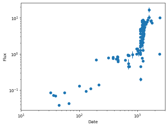
And now you can see our points on the far right! They don’t really make any sense with the trend, but that’s okay because it’s fake data :)